How to save memory by fusing the optimizer step into the backward pass

Hello there! This tutorial aims to showcase one way of reducing the memory footprint of a training loop by reducing the memory taken by the gradients. Say you have a model and you’re interested in ways to optimize memory to avoid Out of Memory (OOM) errors or simply to ooze more out of your GPU. Well, you _might_ be in luck (if gradients take up a portion of your memory and you do not need to do gradient accumulation). We will explore the following:

1. What takes up memory during your training or finetuning loop,

2. How to capture and visualize memory snapshots to determine the bottleneck,

3. The new Tensor.register_post_accumulate_grad_hook(hook) API, and finally,

4. How everything fits together in 10 lines to achieve memory savings.

To run this tutorial, you will need:

• PyTorch 2.1.0 or newer with torchvision

• 1 CUDA GPU if you’d like to run the memory visualizations locally. Otherwise, this technique would benefit similarly on any device.

Let us start by importing the required modules and models. We will use a vision transformer model from torchvision, but feel free to substitute with your own model. We will also use torch.optim.Adam as our optimizer, but, again, feel free to substitute with your own optimizer.

import torch
from torchvision import models
from pickle import dump

model = models.vit_l_16(weights='DEFAULT').cuda()
optimizer = torch.optim.Adam(model.parameters())

Now let’s define our typical training loop. You should use real images when training, but for the purposes of this tutorial, we are passing in fake inputs and not worrying about loading any actual data.

IMAGE_SIZE = 224

def train(model, optimizer):
  # create our fake image input: tensor shape is batch_size, channels, height, width
  fake_image = torch.rand(1, 3, IMAGE_SIZE, IMAGE_SIZE).cuda()

  # call our forward and backward
  loss = model.forward(fake_image)
  loss.sum().backward()

  # optimizer update
  optimizer.step()
  optimizer.zero_grad()

Memory usage during training

We are about to look at some memory snapshots, so we should be prepared to analyze them properly. Typically, training memory consists of:

• Model parameters (size P)

• Activations that are saved for the backward pass (size A)

• Gradients, which are the same size as the model parameters, so size G = P.

• Optimizer state, which is proportional to the size of the parameters. In this case, the state for Adam requires 2x the model parameters, so size O = 2P.

• Intermediate tensors, which are allocated throughout the compute. We will not worry about them for now as they are usually small and ephemeral.

Capturing and visualizing memory snapshots

Let’s get us a memory snapshot! As your code runs, consider what you may expect the CUDA memory timeline to look like.

# tell CUDA to start recording memory allocations
torch.cuda.memory._record_memory_history(enabled='all')

# train 3 steps
for _ in range(3):
  train(model, optimizer)

# save a snapshot of the memory allocations
s = torch.cuda.memory._snapshot()
with open(f"snapshot.pickle", "wb") as f:
    dump(s, f)

# tell CUDA to stop recording memory allocations now
torch.cuda.memory._record_memory_history(enabled=None)

Now open up the snapshot in the CUDA Memory Visualizer at https://pytorch.org/memory_viz by dragging and dropping the snapshot.pickle file. Does the memory timeline match your expectations?

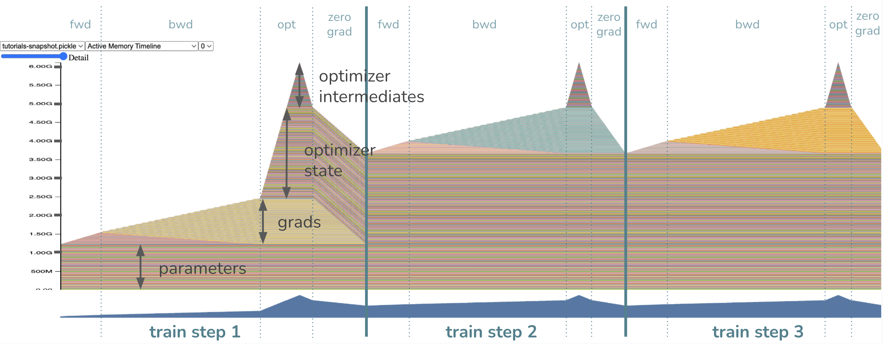
The model parameters have already been loaded in memory before the training step, so we see a chunk of memory devoted to the weights right off the bat. As we start our forward pass, memory is allocated gradually for the activations, or the tensors we are saving to be able to compute gradients in the backward pass. Once we start the backward pass, the activations are gradually freed while memory of the gradients starts building up.

Lastly, as the optimizer kicks in, its state will be lazily initialized, so we should see the optimizer state memory gradually increase during the optimizer step of the first training loop only. In future loops, the optimizer memory will remain and be updated in-place. The memory for the gradients is then freed accordingly at the end of every training loop when zero_grad is called.

Where is the memory bottleneck in this training loop? Or, in other words, where is the peak memory?

The peak memory usage is during the optimizer step! Note the memory then consists of ~1.2GB of parameters, ~1.2GB of gradients, and ~2.4GB=2*1.2GB of the optimizer state as expected. The last ~1.2GB comes from Adam optimizer requiring memory for intermediates, totaling to ~6GB of peak memory. Technically, you can remove the need for the last 1.2GB for optimizer intermediates if you set Adam(model.parameters(), foreach=False) which would trade off runtime for memory. If switching off the foreach runtime optimization is sufficient in memory savings for you, nice, but please read on if you’re curious how this tutorial can help you do better! With the technique we will soon introduce, we will reduce peak memory by removing the need for the ~1.2GB of gradients memory as well as optimizer intermediates memory. Now, what would you expect the new peak memory to be? The answer will be revealed in the next snapshot.

DISCLAIMER: This technique is not for all

Before we get too excited, we have to consider whether this technique is applicable for your use case. This is NOT a silver bullet! The technique of fusing the optimizer step into the backward only targets reducing gradient memory (and as a side effect also optimizer intermediates memory). Thus, the more sizable the memory taken up by the gradients, the more tantamount the memory reduction. In our example above, the gradients eat up 20% of the memory pie, which is quite sizable!

This may not be the case for you, for example, if your weights are already tiny, (say, due to applying LoRa,) then the gradients do not take much space in your training loop and the wins are way less exciting. In that case, you should first try other techniques like activations checkpointing, distributed training, quantization, or reducing the batch size. Then, when the gradients are part of the bottleneck again, come back to this tutorial!

Still here? Cool, let’s introduce our new register_post_accumulate_grad_hook(hook) API on Tensor.

Tensor.register_post_accumulate_grad_hook(hook) API and our technique

Our technique relies on not having to save the gradients during backward(). Instead, once a gradient has been accumulated, we will immediately apply the optimizer to the corresponding parameter and drop that gradient entirely! This removes the need for holding onto a big buffer of gradients until the optimizer step.

So how can we unlock the behavior of applying the optimizer more eagerly? In our 2.1 release, we’ve added a new API torch.Tensor.register_post_accumulate_grad_hook() that would allow us to add a hook onto a Tensor once its .grad field has been accumulated. We will encapsulate the optimizer step into this hook. How?

How everything fits together in 10 lines

Remember our model and optimizer setup from the beginning? I’ll leave them commented out below so we don’t spend resources rerunning the code.

model = models.vit_l_16(weights='DEFAULT').cuda()
optimizer = torch.optim.Adam(model.parameters())

# Instead of having just *one* optimizer, we will have a ``dict`` of optimizers
# for every parameter so we could reference them in our hook.
optimizer_dict = {p: torch.optim.Adam([p], foreach=False) for p in model.parameters()}

# Define our hook, which will call the optimizer ``step()`` and ``zero_grad()``
def optimizer_hook(parameter) -> None:
  optimizer_dict[parameter].step()
  optimizer_dict[parameter].zero_grad()

# Register the hook onto every parameter
for p in model.parameters():
   p.register_post_accumulate_grad_hook(optimizer_hook)

# Now remember our previous ``train()`` function? Since the optimizer has been
# fused into the backward, we can remove the optimizer step and zero_grad calls.
def train(model):
  # create our fake image input: tensor shape is batch_size, channels, height, width
  fake_image = torch.rand(1, 3, IMAGE_SIZE, IMAGE_SIZE).cuda()

  # call our forward and backward
  loss = model.forward(fake_image)
  loss.sum().backward()

  # optimizer update --> no longer needed!
  # optimizer.step()
  # optimizer.zero_grad()

That took about 10 lines of changes in our sample model, which is neat. However, for real models, it could be a fairly intrusive change to switch out the optimizer for an optimizer dictionary, especially for those who use ``LRScheduler``s or manipulate optimizer configuration throughout the training epochs. Working out this API with those changes will be more involved and will likely require moving more configuration into global state but should not be impossible. That said, a next step for PyTorch is to make this API easier to adopt with LRSchedulers and other features you are already used to.

But let me get back to convincing you that this technique is worth it. We will consult our friend, the memory snapshot.

# delete optimizer memory from before to get a clean slate for the next
# memory snapshot
del optimizer

# tell CUDA to start recording memory allocations
torch.cuda.memory._record_memory_history(enabled='all')

# train 3 steps. note that we no longer pass the optimizer into train()
for _ in range(3):
  train(model)

# save a snapshot of the memory allocations
s = torch.cuda.memory._snapshot()
with open(f"snapshot-opt-in-bwd.pickle", "wb") as f:
    dump(s, f)

# tell CUDA to stop recording memory allocations now
torch.cuda.memory._record_memory_history(enabled=None)

Yes, take some time to drag your snapshot into the CUDA Memory Visualizer.

Several major observations:

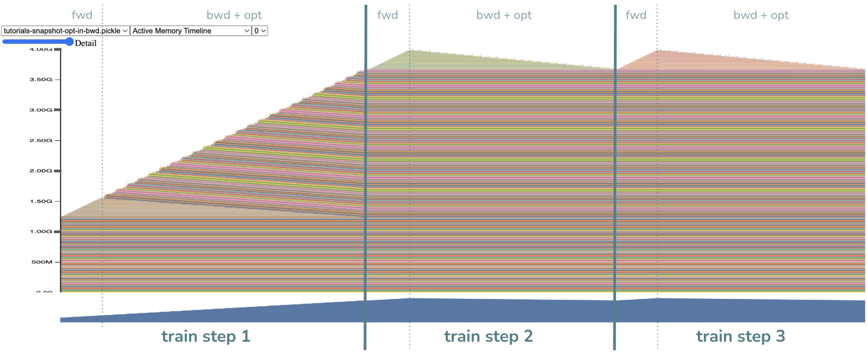
1. There is no more optimizer step! Right…we fused that into the backward.

2. Likewise, the backward drags longer and there are more random allocations for intermediates. This is expected, as the optimizer step requires intermediates.

3. Most importantly! The peak memory is lower! It is now ~4GB (which I hope maps closely to your earlier expectation).

Note that there is no longer any big chunk of memory allocated for the gradients compared to before, accounting for ~1.2GB of memory savings. Instead, we’ve freed each gradient very quickly after they’ve been computed by moving the optimizer step as far ahead as we can. Woohoo! By the way, the other ~1.2GB of memory savings comes from breaking apart the optimizer into per-parameter optimizers, so the intermediates have proportionally shrunk. This detail is less important than the gradient memory savings, as you can get optimizer intermediates savings from just turning foreach=False without this technique.

You may be correctly wondering: if we saved 2.4GB of memory, why is the peak memory NOT 6GB - 2.4GB = 3.6GB? Well, the peak has moved! The peak is now near the start of the backward step, when we still have activations in memory, where before, the peak was during the optimizer step when the activations had been freed. The ~0.4GB difference accounting for ~4.0GB - ~3.6GB is thus due to the activations memory. One can then imagine that this technique can be coupled with activations checkpointing for more memory wins.

Conclusion

In this tutorial, we learned about the memory saving technique of fusing the optimizer into the backward step through the new Tensor.register_post_accumulate_grad_hook() API and when to apply this technique (when gradients memory is significant). Along the way, we also learned about memory snapshots, which are generally useful in memory optimization.